Project 1: Signalized Traffic
The main objective of this project is to design traffic light signal controls in order to optimize particular traffic conditions. Traffic signals regularly pre-establish fixed values red or green for a particular intersection. In fact the behavior can be modeled as:
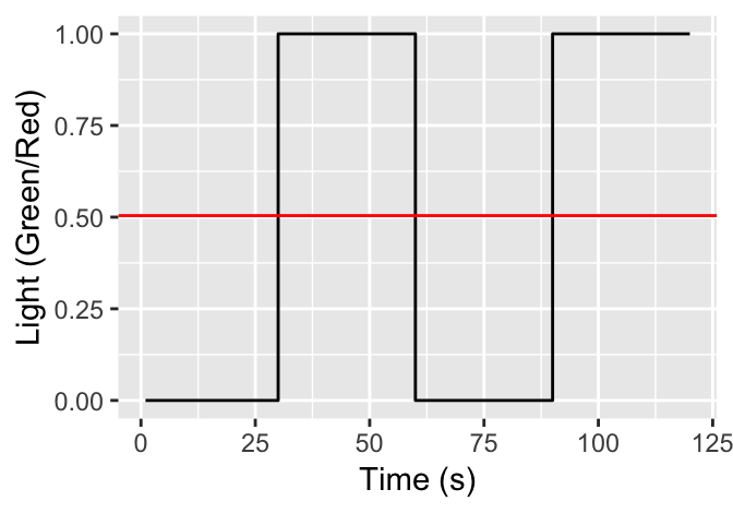
Figure 2: Traffic light signal example.
The relationship between the switched green/red time in a traffic light can be represented by a pulse signal (Figure 2). The red line in the figure represents the duty cycle which represents the fraction of time the light was in green (\(1\)) with respect to the total cycle time (\(60s\)). In this case, the main objective is to study traffic models that can model signalized intersections and design control laws.
Objectives
The main objective of this project is to:
- Study the fundamental aspects of traffic signal control strategies.
- Obtain and simulate a macroscopic traffic model for a urban network with traffic signals
- Create and design control strategies applied via traffic signals in urban traffic networks.
- Compare the behavior of fixed-time traffic signal polices and dynamic-time traffic signal polices.
Description
Task 1: Modeling
Check models for macroscopic networks: (Grandinetti, Canudas-de-wit, and Garin 2015), (Grandinetti, Garin, and Canudas-de-wit 2015),(Varaiya 2013). Determine the parameters required to model a road traffic network.
Context
Before implementing a real scenario in this phase we aim to describe the context of a virtual example. Consider the following traffic urban corridor which obeys a simplified version of the real arterial scenario.
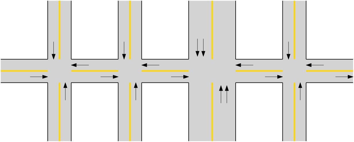
Figure 3: Example of traffic network.
The network of Figure 3 represents a regular corridor in a city like. The priority for this type of corridors is to maximize the priority of green time so the traffic does not get congested along the network. It is important to highlight that for the proposed network
Questions
- Based on a literature review, determine current existing traffic models for signalized traffic networks.
- For the network in Figure 3, build a macroscopic signalized traffic model.
- Determine the signalized/averaged traffic model for the case where lights are installed along each intersection of the corridor. For those roads in which direction is not explicitly defined, consider the direction of a regular intersection.
Expected outcomes
Present a brief summary of the existing current models for signalized traffic networks. At same time highlight the key features of these models and the remaining difficulties. Consider including references for the presented models.
Based on (Grandinetti, Canudas-de-wit, and Garin 2015) obtain a model for the signalized network of Figure 3 and the parameters required model this corridor.
Define the set of parameters for the traffic network, notably those related to the fundamental diagram as well as the traffic light signal timings. Consider a fixed setup of this parameters for the moment and overall explain the reason of the choice.
Task 2: Simulation
Dynamic simulation of open loop traffic networks. For this task be sure to review already implemented simulations available at Link. Get familiar with the code here developed before you enter into details of implementation.
Context
Based on the model established in the Task 1 and considering a family of specific parameters, perform a simulation for a constant demand value of demand in \(veh/hr\) as specified in the Figure4.
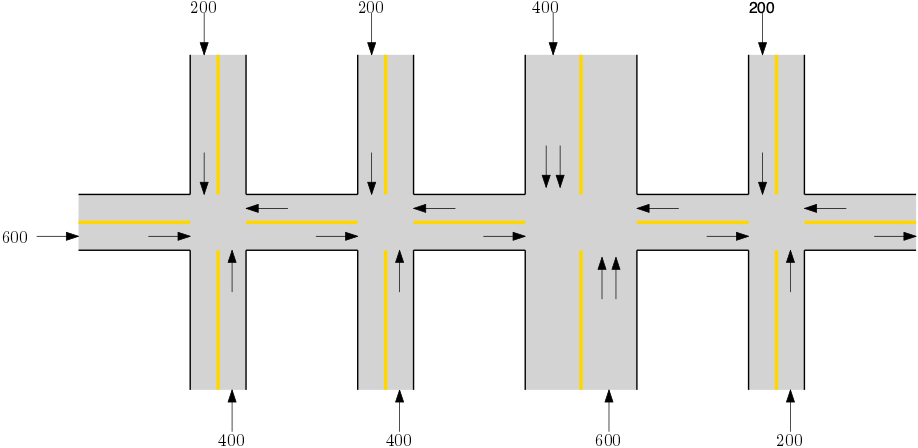
Figure 4: Demand profiles for a specified scenario.
Questions
Simulate and obtain density plots of the dynamic the behaviour when the duty cyle of lights is similar for all the traffic lights. \(50\%\)
Does the current values create a congestion in the proposed network?
How can the performance of the network be improved? Create a second set of parameters for the traffic lights duty cycle
For the existing model and according to (Grandinetti, Canudas-de-wit, and Garin 2015) obtain the two different density and flow dynamic profiles between a switched signalized traffic model and an averaged traffic model
Expected outcomes
Present the dynamic profiles for density on each one of the roads under different setups of traffic lights. The dynamic profiles should specify density per road in time
Provide comparisons between different traffic signalized models and an analysis on how this error evolves according to different values of demand.
Specify a second set of parameters for duty cycle that could improve the performance of the network with respect to the \(50\%\) case. Justify the reason of your choice and verify in results the desired behavior.
Task 3: Control strategy
For this task we aim to consider the duty cycle as a control input variable to regulate the flow within the traffic network. In this case take into account that the decision variable needs somehow to be determined dynamically via a control algorithm.
Context
For the Figure 2 the average value can be found as:
\[\begin{equation} \bar{u} = \frac{1}{T}\int_0^T u(\tau) d\tau \tag{1} \end{equation}\]As it is illustrated in (Grandinetti, Garin, and Canudas-de-wit 2015), in Eq. (1) is easier to design a value for \(\bar{u}\) rather than \(u\) due to its binary character.
Questions
Explain and construct a block diagram illustrating the control of the road traffic network via traffic signals
Design and present an algorithm that takes decisions for the traffic signals based on the state of the network. How would you construct the value of \(u\) based on the congestion state of the network.
Perform simulations of the system under a preestablished manual control and compare it to a situation where the control depends on the congestion state of the network.
Expected outcomes
Present a comparison between the traffic network with signalized control and without signalized control.
Apply the controller over different versions of the model notably averaged and switched
Compare the open loop situation with the closed loop situation and provide conclussions on the control performance.
Task 4: Performance evaluation
Finally in order to compare it is important to determine indicators than can be designed in order to compare the effects of introducing an automated control strategy.
Context
Indicators for traffic networks are regularly expressed in terms of the state of the network, for example the Service of Demand (SoD) measured in terms of flow:
\[\begin{equation} SOD = \int_0^T \sum_{r \in R} f_r(\tau) d\tau \tag{2} \end{equation}\]Or the Total Travel Distance (TTD) measured in terms of the density
\[\begin{equation} TTD = \int_0^T \sum_{r \in R} \rho_r(\tau) d\tau \tag{3} \end{equation}\]Questions
What does the aforementioned indicators represent?
Measure the indicators over the traffic network with a manual setup of traffic signals open-loop vs a controlled setup of traffic signals closed-loop.
Expected outcomes
Report indicators for both cases and conclude about the results.
Provide recomendations on how to design \(u\) for the corridor
References
Grandinetti, Pietro, Carlos Canudas-de-wit, and Federica Garin. 2015. “An efficient one-step-ahead optimal control for urban signalized traffic networks based on an averaged Cell-Transmission Model.” In 2015 European Control Conference (Ecc), 3478–83. Vienna, Austria: IEEE. doi:10.1109/ECC.2015.7331072.
Grandinetti, Pietro, Federica Garin, and Carlos Canudas-de-wit. 2015. “Towards scalable optimal traffic control.” In 54th IEEE Conference on Decision and Control (CDC 2015). Osaka, Japan. https://hal.archives-ouvertes.fr/hal-01188811.
Varaiya, Pravin. 2013. “Max pressure control of a network of signalized intersections.” Transportation Research Part C: Emerging Technologies 36 (2). Elsevier Ltd: 177–95. doi:10.1016/j.trc.2013.08.014.